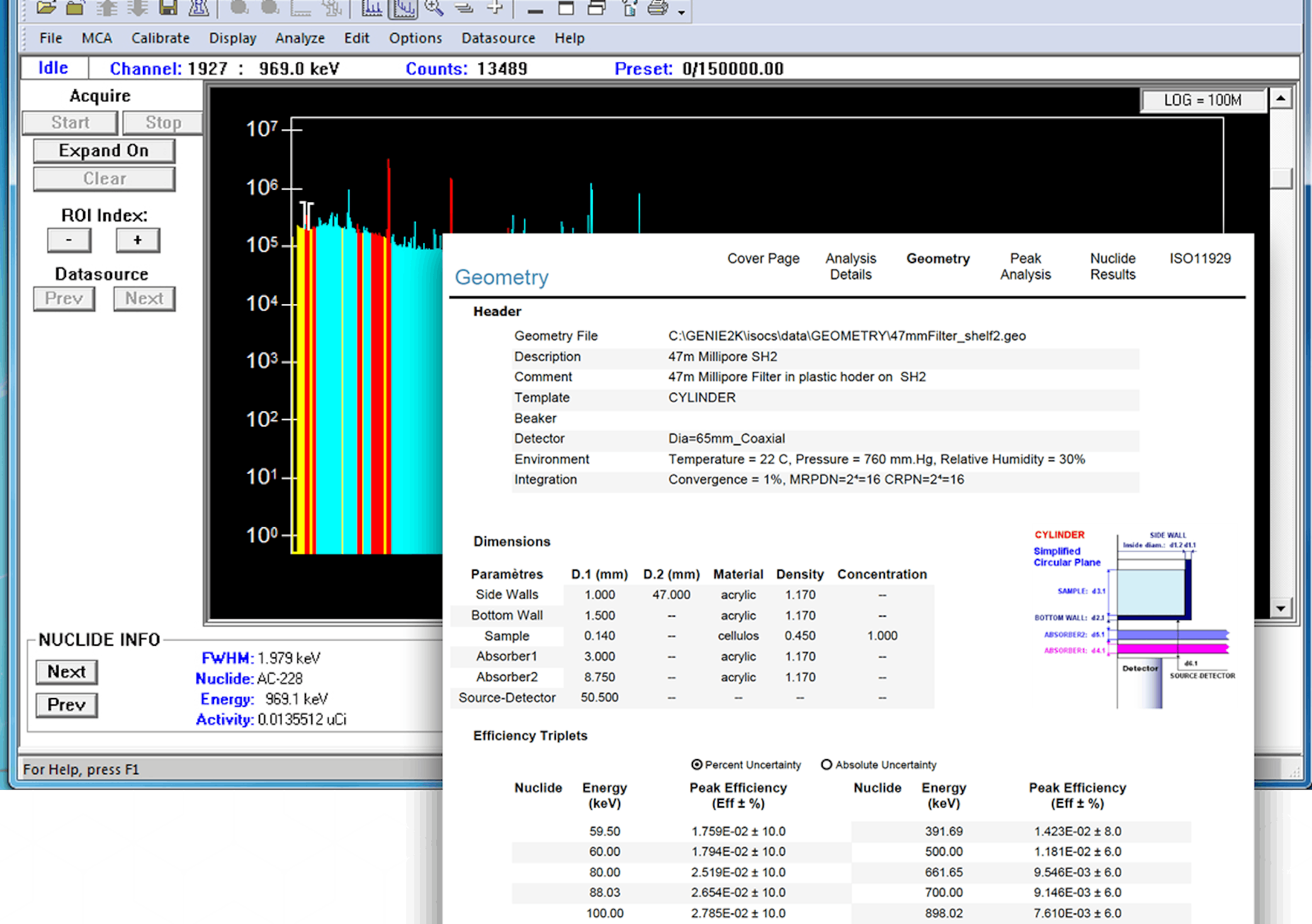
REGIONAL ACCESS
USA ---------------------- Benelux Canada France Germany Japan Northern Europe Russia United Kingdom

EXTRANET ACCESS
select a site ---------------------- CINET Extranet HIS-20 Extranet HP SW Updates

Introduction

Every component in a Ge Gamma Spectroscopy System, from the detector through the MCA system, has its own unique count rate limitations. Fortunately, thanks to today's technology, these count rate limits are fairly high. At modest count rates - under a few tens of kHz - obtaining precise, accurate results from a gamma spectroscopy system is a relatively routine task.

At higher rates, however, things aren't quite so straightforward. Problems like loss of resolution, excessively long counting times, erroneous peak to background ratios, inaccurate counting statistics, or even system shutdown due to overload and saturation, start to appear. And not only do these problems appear, but their nature and severity can vary from one type of sample to the next! In short, at very high count rates, precise, accurate gamma spectroscopy can quickly become anything but routine.

In this note we'll be looking at these various count rate related problems, the specific limitations that each component imposes on overall system performance, and how these limitations might be overcome. In addition, since there will usually be no one universal solution to a given set of problems, we'll be closely examining the count rate, resolution, and pricing trade-offs that are available and how they can be optimized to build cost-effective systems tailored to specific applications.

What are the System Count Rate Requirements?

Generally speaking, high count rate considerations come into play when dealing with samples with higher levels of radioactivity. The higher the activity, the higher the incoming count rate.

But to determine whether or not special measures should be taken in the selection of system components, you need to look more closely at the end objective - the measurement being taken.

Spectroscopists often refer to "high count rate" applications when what they mean is "high incoming count rate". While high incoming count rate applications certainly raise problems of their own, they are quite different from those requiring high throughput.

As we will see in the subsequent discussions, raising system throughput capability almost inevitably degrades system resolution. Since resolution is often more critical to measurement quality than the number of counts in spectral peaks, optimizing for throughput may not be the best solution for all applications involving hot samples.

In many applications, "low" throughput components function quite nicely in a high count rate environment. It may take longer to accumulate a spectrum with desired statistics, but the resolution will often be superior.

The spectroscopist can take a number of measures to reduce the count rate coming into the system - preserving system resolution while still getting high quality data. Samples can be diluted or collimators can be placed around the sample to reduce the total number of photons striking the detector. Or a smaller (and fortunately, less expensive) detector can be selected to reduce the number of events that need to be processed by the system.

If the application has high incoming count rates and requires high throughput - large numbers of events processed in a short time - then the techniques described in the rest of this note will guide you towards the optimum solution. Even if throughput is not a concern, this note will assist in the selection of the best components for handling high incoming count rates irrespective of the throughput considerations.

Some Basic Terminology

Before we can look into the specifics of what are generically called "count rate problems", we'd better make sure we are all talking the same language. To that end, four very important terms that you will see throughout this note and what, exactly, is meant by them will be briefly reviewed.

Operating Limit:

The energy or count rate beyond which a given component in the system ceases to function. While this figure may be of interest, what really matters is...

Throughput Rate:

The maximum rate at which a given component (or system) can process or analyze counts in a valid manner.

Count Rate Limitation:

A performance limitation related strictly to the number of input counts (events) per unit of time, regardless of the energy of those events.

Energy Rate Limitation:

A performance rate limitation related both to the number of events per unit of time and the energy of those events. (e.g., an Energy Rate limited component might be capable of processing 500000 low energy events per second but only 100000 high energy events per second.)

Keeping these definitions in mind, we'll start our discussion with an overview of the major components in a Ge Gamma Spectroscopy System and the general nature of their throughput limitations.

System Component Throughput Limits

The basic components of a Ge Gamma Spectroscopy System, together with their typical throughput limits, can be seen in Table 1. In this section we will take a quick look at just what these mean. In the sections which follow we'll cover each component in detail, the goal being to better understand just how each can be optimized for high count rate applications.

The Detector

The first thing you'll notice is that the detector is the least of your worries when it comes to handling high count rates, for its throughput capability is several times greater than any of the other components in the system. It's very fortunate that this is the case, for the limitation is due to the laws of physics; the amount of time it takes the signal from an event to travel through the germanium (the Charge Collection Time) determines the limit, and for a given detector there's really not much you can do about it.

The Preamplifier

The preamp, you'll notice, is Energy Rate Limited. That is, its throughput capabilities decrease as the energy of the events it is processing increases. In addition, the most commonly used preamplifiers (RC Feedback Type) have an absolute Operating Range limit, and when they reach that limit they simply stop working.

As we'll see later when we examine preamps in detail, there are some resolution trade-offs that can be made that will greatly increase an RC preamp's energy limit, and there are certain types of preamps (Transistor Reset Type) that - while having a lower overall throughput capability - don't have a "shutdown" problem when they reach their upper limit.

The Amplifier

The spectroscopy amplifier is one of the weakest link in the system's throughput capabilities. And in general, anything you do to the amp to improve its count rate capabilities will do so only at the cost of decreased resolution. Gated Integrator type amplifiers offer a possible solution, and they - together with the count rate and resolution trade-offs involved - will be covered in detail in a later section.

The Analog to Digital Converter

Though relatively expensive, the fastest of today's Fixed Conversion Time (FCT) ADCs are able to keep up with just about any count rate that the remainder of the system can handle. But if you have to use a Wilkinson type ADC because that's what you own - or if you prefer the Wilkinson ADC because of its generally better linearity and resolution performance - the throughput of the ADC can be a factor.

In Table 1 you'll see that Wilkinson ADCs, like RC Preamps, are energy rate limited; the lower the energy the higher the throughput capability. In fact, if you are analyzing primarily low energy samples, you may find that a lower cost Wilkinson ADC may actually outperform all but the fastest of the FCT ADCs.

In our detailed look at ADCs the benefits and limitations of both types will be discussed, and application specific recommendations made.

Table 1 Major System Components and Their Throughput Limitations

The MCA

The last component in the system is the MCA, and unless it is an older model or a relatively low cost unit, it should not be a limiting factor in your system's throughput capabilities. However, the specific MCA that you use may place a limit on the types of Live Time Correction that are available to you, so some discussion on the alternatives that are available is in order.

Live Time Correction

Though more of a process than a component, compensating for the throughput limitations of the system - which is what Live Time Correction really does - is a major concern. If it's not done correctly and accurately the results of your analyses will be - in a word - wrong. Both hardware and software corrections will be examined, and specific recommendations made for various applications.

Having taken a quick look at the elements which make up a system, we'll now study each in greater detail.

The Germanium Detector

As was pointed out earlier, the detector is the least of your worries when it comes to throughput bottlenecks in a Ge Gamma Spectroscopy System. Unless you have an extremely large high efficiency Ge detector, the detector will usually be capable of handling count rates several times greater than the weaker links in the system. However, with extremely large detectors - which are really more suited to environmental, rather than high count rate, samples - detector dead time could become a factor, so it's worth spending a few minutes discussing the cause of the detector's count rate limitations: Charge Collection Time.

Charge Collection Time and Pulse Pileup

A diagram of a standard coaxial Ge detector is shown in Figure 1. When a photon interaction takes place (an event is detected), charge carriers in the form of holes and electrons are produced. The electrical field produced by the detector's high voltage bias supply causes these carriers to be swept toward the P and N electrodes of the detector. The time it takes the carriers to travel to the electrodes is called the Charge Collection Time. Charge carriers move at rate of about 1 mm/10 ns, so in a good sized Ge like the one shown, with an average path length of 25 mm or so, the Charge Collection Time would be about 250 ns. This yields a Count Rate Limit of approximately 4 MHz.

Figure 1 Ge Detector Charge Collection

But what happens at higher rates? Actually, the detector keeps on working at even higher rates, but the data isn't any good! Should a second (or third) event take place while the first set of charge carriers are still in transit, the energy from the two events get added together. That is, should a 2 MeV event arrive while a 1 MeV event is in transit, the detector would "see" a single 3 MeV event, producing a sum peak. When the detector starts reporting more sum peaks than valid events, you have exceeded its count rate capability.

As we'll see later, Charge Collection Time and Pulse Summing or Pileup can also cause peak shape and risetime problems. But the real upper limit to a detector throughput is the summing we just discussed.

Is There an Answer?

Should this be a problem in your application, what can you do about it? Basically you only have two choices:

1. Reduce the number of events the detector "sees": move the sample further away or collimate the detector.
2. Use a smaller, less efficient detector; the smaller the detector the lower the charge collection time, which means a higher count rate limit.

Note that since method two requires the use of a less efficient detector it also reduces the number of events that the detector will "see", so both methods are essentially equal in impact. Choose the one that best fits your application configuration and budget.

The Preamplifier

Most germanium detectors in use today are equipped with dynamic charge restoration, or RC feedback, charge sensitive preamplifiers. These preamps are relatively inexpensive and offer very good resolution, making them an excellent choice for low to moderate count rate applications. However, as was mentioned earlier, RC preamps are energy rate limited and have an upper limit that, when exceeded, causes them to saturate and bring system throughput to a standstill. Because of the potential severity of this problem, time invested in exploring the cause and some possible solutions will be time well spent.

Basic Preamplifier Operation

In Figure 2 you'll see a schematic of a typical Ge Detector and RC Feedback Preamplifier. The output of the preamp, as measured at the test point, is shown in Figure 3 for two different count rate scenarios.

Figure 2 Typical RC Feedback Preamplifier

The preamp output, you'll notice, is a tail pulse. The information (energy of the detected event) is carried in the amplitude of the pulse. The tail contains no information; it is there simply because it takes a finite amount of time for the Feedback Resistor in the preamp to discharge the circuit back to ground state.

As you can see in Figure 3A, the arrival of a second pulse prior to the first completely decaying is normally no problem; it rides upon what is left of the tail of the first pulse. This will cause the average dc level of the signal baseline to rise slightly, but as long as the sum of any residual tailing plus the amplitudes of the pulses being processed does not exceed the dynamic range of the preamp, all is well. The dynamic range, it should be pointed out, is a function of the preamp power supply voltage and is nominally 20 volts or so for most RC feedback preamps.

Figure 3B represents a case of preamp saturation; the events are coming at such a rate and with such a high energy that the dynamic range is exceeded. At this point the preamp stops operating, and will stay dead until the incoming energy rate slows down sufficiently to allow the feedback resistor to draw the baseline dc level down to within the operating range.

Figure 3 RC Preamp Test Point Output at Varying Count Rates

The real crux of this problem is the decay time of the tail pulses, and that time is directly related to the value of the feedback resistor. One way to decrease that time, which will increase the energy throughput rate, is to lower the value of the feedback resistor.

While that does indeed work, there is no such thing as a free lunch; as you decrease the resistance from its typical 2 Gigohm value you also increase the noise in the preamp, which degrades the resolution of the detector.

The Transistor Reset Preamp Alternative

A better solution to this preamp saturation problem is to use something called a Reset Preamplifier. In this instrument the feedback resistor is replaced with a reset circuit that monitors the dc level of the preamp and discharges the feedback capacitor whenever it starts to approach saturation.

At moderate to high count rates - above a few tens of kcps - the Transistor Reset Preamplifier (TRP) offers the Germanium Gamma Spectroscopist two distinct advantages in comparison to traditional Resistor Capacitor (RC) Feedback type preamplifiers:

1. Improved Resolution. By eliminating the feedback resistor and its attendant noise and secondary time constant contributions, TRPs offer inherently better resolution and reduced spectrum broadening at high count rates.
2. Increased Count Rate Capability. TRPs are not energy rate limited like RC type preamps, so they virtually never shut down due to saturation; at even the highest of count rates some pulses will always get through.

Throughput & Resolution Optimization

We tested a traditional RC preamplifier and a Transistor Reset Preamplifier to compare the performance of the two technologies. We started with two very closely matched high resolution germanium detectors, one fitted with our 2002 RC preamplifier and the other with our model 2101 Transistor Reset Preamplifier. Next we selected two amplifier/ADC configurations. One optimized for throughput and the other for resolution.

1. The High Throughput System consisted of our Model 2024 Gated Integrator Amplifier with 0.25 µs shaping time and Model 8715 800 ns, Fixed Conversion Time ADC.
2. The High Resolution System used our Model 2025 AFT Research Amplifier with a 2.0 µs shaping time and our Model 8706, a 450 MHz Wilkinson ADC.

First we tested each of the two preamplifiers with the high throughput system and then with the high resolution system. Since the same configurations were used to compare the two preamplifiers, in each case, any differences in test results must be due to the preamps themselves. In the following sections we review the test results to see just what sort of impact a TRP has on the performance of a gamma spectroscopy system.

Throughput

The results of the throughput tests can be seen in Figure 4, and they clearly show the benefit of a TRP at extremely high count rates. Long after the RC preamp has shut down due to energy rate saturation the TRP is still working quite nicely! In fact, with a TRP the real limitation is pulse pileup in the Amp/ADC, which is the reason the throughput curve drops off just beyond a 200 kcps input rate.

Figure 4 Throughput vs. Count Rate: Throughput Optimization (2024 GI at 0.25 µs, 582 ADC)

Note, however, that at its peak the RC preamp actually has slightly better throughput - by 5 to 10% - than the TRP. This is due to the added deadtime the TRP's resetting process adds to the total system deadtime (more on this later), and is the cost of using a TRP. Since that cost is only a few percent with the 2101/2024 Preamp/Amp combination, it would seem to be a reasonable price to pay for added count rate capability.

Resolution

Figure 5 shows the resolution performance of the preamplifiers using the Gated Integrator high throughput configuration. Note that while the two preamplifiers start out with equal resolution, the TRP's design results in much less resolution degradation than the RC preamp as the count rate increases. The TRP does not require a feedback resistor. As a result, the associated parasitic time constants are eliminated, allowing improved performance at high count rates. The higher the count rate the more evident the TRP advantage.

Figure 5 Resolution vs. Count Rate: Throughput Optimization (2024 GI at 0.25 µs, 582 ADC)

The TRP Reset Process

While the TRP never completely shuts down due to saturation, its reset process and the amplifier overload which it causes does induce intervals of dead time into the counting system. Depending upon the nature of the sample being analyzed and the specific preamp/amp combination being used, these dead time intervals can be as insignificant as a couple of µs every few hundred pulses or as great as hundreds of µs every ten pulses.

While the former situation, which adds only a few percentage points to the system dead time, may be a very reasonable price to pay for the throughput and resolution benefits gained with a TRP, the latter could be a dead time nightmare.

It's the resetting process itself that causes deadtime when a TRP is used, so that's the area we'll examine in some detail.

The output of a TRP can be seen in Figure 6, and there are several very important characteristics to note:

1. The output is a step function, rather than the tail pulse associated with an RC preamp. This means that pole/zero cancellation is not required in the amplifier.
2. The Dynamic Range of the preamp output is much lower than that of an RC preamp (the Reset Threshold of most TRPs is 4 volts; in most RC preamps, the Saturation Level is 20 volts or so).
3. When the output of a TRP reaches its reset threshold, it is automatically reset. There is no saturation and for most applications, no energy rate limit.

Figure 6 The TRP Reset Process

This resetting process, which is the secret to being "never dead", takes time. The time required to reset contributes to overall system dead time.

To minimize system deadtime, two steps should be taken:

1. Choose a TRP with the widest possible dynamic range. This basically allows more pulse steps to occur before reset is required.
2. Choose an amplifier with the best possible overload recovery characteristics.

Preamp Summary

Transistor Rest Preamps, in both throughput and resolution optimized system configurations, do indeed outperform standard RC type preamps: TRPs are not energy rate limited, and they exhibit much better resolution and spectrum broadening characteristics.

While there is a deadtime "cost" to be paid to gain these advantages, selecting an optimum TRP/Amp combination can keep that cost low enough to make the price you pay for the added performance well worth it.

The Spectroscopy Amplifier

As we've just seen, it's possible to raise the throughput capabilities of your system by choosing the right preamp without sacrificing system resolution. Having done that, the weak link in the throughput chain is now the spectroscopy amplifier. In this section we'll be examining the reasons behind the limitations in spectroscopy amplifiers and how they might be overcome.

Basic Signal Processing

Signal processing, rather than simple amplification, is really what a spectroscopy amplifier does for a living. It extracts the energy (and timing) information from the preamp's output and converts it to a form that can be easily analyzed by an ADC. The three basic stages of the process can be seen in Figure 7.

Figure 7 Amplifier Signal Processing

From the last section the long tailed pulses and the floating baseline of the preamp signal in Figure 7A should look familiar. One of the problems in analyzing signals of this type is that there is no common baseline reference, so the first thing a spectroscopy amplifier does is use a differentiator to clip the signal to a faster fall time and block the low frequency or dc components in the input signal.

Since the differentiator is essentially a high pass filter, the energy information contained in the leading edge of the signals is passed through and the tailing sharply clipped to the baseline. The result of this process can be seen in Figure 7B. It's usually done in the early stages of the amplifier for the faster signal fall times reduce the effects of overload and pileup on the remainder of the amplifier circuitry.

Next comes an integrator (low pass filter), which is used to recover the energy information from the signal. This yields the Gaussian shaped pulses shown in Figure 7C. The amplitude of each pulse is directly proportional to the energy information content of the associated preamp tail pulse.

Figure 8 shows one such pulse in detail. Measuring from the 0.1% points, a typical spectroscopy amplifier will produce a near Gaussian shaped output that is 7.3 shaping time constants in width with a time to peak of 2.4 shaping time constants.

Figure 8 The Amplifier Output Pulse

The Role of the Shaping Time Constant

Though selective frequency active filters are actually used to do these differentiation and integration tasks, the roll played by the Shaping Time Constant (TC) can best be seen if you "pretend" that simple RC networks are used.

For the differentiator, shorter time constants mean higher throughput, for they will pull the tail of the preamp pulses down to the baseline more quickly. Unfortunately, shorter TCs also mean that the integrator will pass more high frequency noise, degrading the quality of the signal. In addition, particularly with very large detectors, a shaping TC that is too short will allow a phenomenon known as Ballistic Deficit to start degrading the resolution of the data.

Charge Carrier Ballistics

Ballistics has to do with the nature of the motion of charge carriers in a detector. Referring back to Figure 1, the path taken by the charge carriers for that particular photon event are shown by dotted lines. The length of the two paths are about the same, so - assuming that the electrical fields in the detector are uniform - the holes and electrons will both get to their respective electrodes at about the same time. This is what you wish would always happen, for this yields preamp pulses with nice short rise times in the area of a few tens of nanoseconds.

In reality however, the photon interactions can take place anywhere within the active volume of the detector. Should an interaction occur very close to one of the electrodes, the two paths will be very different in length. Assuming the same 25 mm path length we used earlier, one set of carriers might only have to travel a millimeter or so, meaning that the other set has to cover more than 20 mm. At a travel rate of around 1mm/10 ns, it will take the second set of carriers over 200 ns to reach their electrode.

Since the charge collection isn't finished until the last of the carriers have completed their travel, this will yield a preamp pulse risetime of over 200 ns. With really large detectors (>75% Relative Efficiency), the worst case can be several times that. Because of this phenomenon, the pulses from a preamp really look like the ones in Figure 9; each pulse will have a different risetime depending just where within the detector the associated interaction took place.

Figure 9 Preamp Risetime Variations (Greatly Exaggerated) Due to Charge Carrier Ballistics

But what does this have to do with the shaping time constant? Experience has shown that, to fully process a pulse from the preamp, the TC needs to be about 10 times the risetime of the input pulse. If it's not, you effectively stop processing the pulse before it has risen to its maximum amplitude. This means that the amplitude of the amplifier's output pulse will be too low, which means loss of resolution in the data. This pulse height distortion, which is caused by using a TC that is too short, is called the ballistic deficit.

Because of the "times 10" rule just mentioned, for most Ge detectors a 2 µs TC is the smallest that can be used if ballistic deficit is to be avoided. And with very large detectors, where the charge collection paths and total travel time are much longer, 4 µs is the minimum.

Pulse Pileup

Based upon the above discussion, it would seem like erring on the side of a slightly too long of a TC would be the best compromise. And it is, if maximum resolution is the only concern. But longer time constants mean longer amplifier processing time, and that reduces the throughput capabilities of the amplifier.

This reduction shows up as pulse pileup, which can be seen in Figure 10. When a new pulse from the preamp arrives before the amplifier has had a chance to process the previous pulse, a summing takes place. This appears in the form of pulses piled on top of one another, with no return to the baseline reference between the pulses. And because of the summing, the piled up pulses are really invalid events, for their amplitude - compared to the baseline - bears no relationship to the actual events.

While, as we'll see later, there are ways to prevent these invalid events from being processed so they won't distort your data, the net effect is decreased system throughput.

Figure 10 Pulse Pileup

Shaping Time Constant Tradeoffs

Just as in the case of the preamp feedback resistor, there are resolution vs. throughput tradeoffs that can be made in selecting the shaping time constant to be used for a given application. Figure 11 illustrates the points that will be covered.

With a 2 µs time constant, the value recommended for good resolution and reasonable throughput with most Ge detectors, the maximum throughput capability is just under 20 kcps. This is achieved at an input count rate of about 40 kcps, and if the input rate exceeds that value, throughput actually decreases due to pulse pileup.

As you can see in Figure 11A, going to a 1 µs TC almost doubles the amplifier throughput, and the peak throughput is not reached until the input rate approaches 100 kcps. But there is a price for that extra throughput: decreased resolution.

Figure 11B shows the effect of the TC on resolution for a typical small coaxial Ge detector. If the ⁶⁰Co resolution was 1.8 keV at 2 µs shaping, you can expect about 2.2 keV at 1 µs. That's a degradation of over 20%, which is a lot. But it hasn't been all that many years since a 2.2 keV detector was considered to be a pretty good one, so unless you have an extremely complex sample the tradeoff to get double the throughput may be a very good one.

Figure 11 Resolution vs. Throughput Tradeoffs for a Standard Spectroscopy Amplifier

The Gated Integrator: Turbocharged Gamma Spectroscopy

If you can afford to give up a few more tenths of a keV in resolution, "turbocharging" your spectroscopy amplifier with a Gated Integrator (G.I.) can more than double your throughput.

To see just what you gain and what it costs, take a look at Figure 12, where the performance of a G.I. using 0.25 µs shaping has been added to the throughput and resolution curves of a standard spectroscopy amplifier. If you can tolerate your 1.8 keV detector performing at a 2.4 keV level, you'll easily handle incoming count rates of about 200 kcps and successfully process around 70 kcps through the amplification system.

Figure 12 The Gated Integrator vs. a Spectroscopy Amplifier.

A gated integrator, like a turbocharger, is an accessory for the main spectroscopy amplifier "engine". To see just how it works, particularly since it utilizes a very short amplifier shaping time constant to gain its added throughput, we have to look again at a ballistically deficient Gaussian output pulse.

The unipolar pulse in Figure 13 is ballistically deficient; that is, because the shaping TC of the amplifier was too short the amplitude of the Gaussian pulse is too low. In addition, the pulse has a noticeably long tail. And it is in this tail that the energy that was "lost" from the peak amplitude can be "found". In other words, while the energy represented by the peak's amplitude is incorrect, the area of the peak contains a true representation of the energy content of the pulse from the preamp.

Figure 13 Unipolar vs. Gated Integrator Outputs

The gated integrator's role, then, is to integrate the area of these deficient peaks to produce an output peak whose amplitude is proportional to the area of the unipolar pulse. And since we just saw that the unipolar peak area is proportional to the energy from the preamp's pulse, the result from the G.I. is what we've been trying to achieve all along: a pulse whose amplitude is proportional to the energy of the event that the detector captured! Ballistically deficient peaks have now been turned into valid events, allowing us to use shorter TCs for greater throughput.

A fairly simple concept, actually, and one that works well. But there is a price to pay. As you can see in Figure 12B, with most detectors the resolution does get degraded slightly when compared to a standard amplifier using a 1 µs or greater shaping time constant. This is due to the extra noise that the shorter G.I. shaping time constant lets through the amplifier, and is the cost of the added throughput that is gained.

It should also be noted that a Gated Integrator is really a special purpose instrument designed for very high count rates. At normal count rates, where very short shaping times aren't required, the resolution of a G.I. is never quite as good as a standard spectroscopy amplifier (see Figure 12B). For that reason, gated integrator amplifiers which include a switch to disable the G.I. and allow for normal amplifier operation at moderate counting rates are more versatile.

Pulse Pileup Rejection

As we saw in the previous section, pulse pileup occurs when a new pulse from the preamp reaches the spectroscopy amplifier before the amplifier has a chance to finish processing the previous pulse (see Figure 10). While the use of shorter shaping time constants minimizes pileup, there will always be some upper incoming count rate limit beyond which the amplifier will produce more piled up events than valid events. This is the reason that the throughput curves in Figure 11A, for example, build up and then start to decrease.

Assuming a properly set up amplifier, there is no way to avoid pileup other than reducing the incoming count rate. But there is a way to insure that piled up events, which are invalid and simply increase the apparent background of the spectrum, are not processed by the system's ADC.

The circuit which does this for us is called a Pileup Rejector/Live Time Corrector (PUR/LTC), and any spectroscopy amplifier suitable for high count rate Ge spectroscopy will include one. As you can see in Figure 14, they are extremely effective. At high count rates you can expect the background contribution from piled up events to be reduced by close to two orders of magnitude. And best of all, it does this for "free"; there are no resolution or throughput tradeoffs involved. It simply improves your data, making the spectrum easier to analyze and giving it better counting statistics.

Figure 14 PUR Operation, 57Co at 80 kcps and 4 ms Shaping

The Pileup Rejector

The basic concept behind pulse pileup rejection is very straightforward: if a new pulse arrives from the preamp before the amplifier has finished processing the previous pulse, the PUR generates a Reject signal. This tells the data acquisition system that the event is invalid and should be ignored.

While there are several different ways in which the circuitry can be physically implemented, the logical operation of a PUR can be seen in Figure 15. Reject Signals (R1 and R2) are only generated and sent to the ADC when Preamp Pulses (P3 and P5) come along prior to the Amplifier's Unipolar Output (A2 and A3) returning to the baseline.

Figure 15 PUR/LTC Signals and Timing

Trailing Edge Pileup

The ADC, however, cannot blindly reject data every time it gets a Reject signal. For example, consider Amplifier Pulse A2. Because of the way in which the peak detector works in an ADC, the event on the leading edge pulse A2 is valid; that is, it started at the baseline, rose to its maximum amplitude, and started back down again. In the ADC, once a pulse has risen from its baseline to its peak and returned back to its 90% point the ADC is happy and accepts the event for conversion, as it should. This process is called Peak Detection, and the time required to perform it is the ADC's Linear Gate Time.

Directly below Amplifier Pulse A2 you'll see the associated ADC Linear Gate signal G2, which ends at Time Line 7. Since it ends before the trailing edge pileup and associated Reject signal R1 is generated, the ADC ignores the Reject and properly converts the event. Since this event does not return to its baseline before the piled up pulse on its trailing edge begins, the ADC never sees the piled up pulse and therefore doesn't process it.

Leading Edge Pileup

Next take a look at Amplifier Pulse A3, the associated Linear Gate Signal G3, and Reject signal R2. Since the Reject is generated before the ADC has detected a peak - Linear Gate is still true at Time Line 11 - this event is indeed invalid and will be rejected.

The Live Time Corrector

Live time correction (or more properly, dead time compensation) has been traditionally viewed as something only the ADC had to worry about. But when you use a PUR, amplifier deadtime - and hence compensation for it - becomes a factor.

The PUR/LTC generates a Dead Time Signal and sends it to the ADC. There it gets ORed with the ADC's own Dead Time Signal to insure proper compensation when either the ADC or the Amp are busy or the pileup rejector has decided that the ADC should not process a pulse.

The very last signal in Figure 15 is the Dead Time signal generated by the PUR/LTC. It begins when an event from the preamp is detected, and ends when:

1. The ADC has processed a valid event, as indicated by the Linear Gate interval ending prior to any Reject occurring, and
2. The associated Amplifier Output returns back to the baseline.

When there is no pileup, this signal simply represents the time during which the amplifier is busy processing a pulse, as shown by DT1. In the case of Trailing Edge Pileup (A2 and DT2) this is also what happens.

But now look at DT3. Because of the "ending rules" just mentioned, the PUR/LTC Dead Time gets stretched out from the start of Preamp Pulse P4 until Amplifier Pulse A4 returns to the baseline. This is necessary due to the random, as opposed to periodic, nature of the pulses being processed. Though the statistics to prove it are beyond the scope of this note, accurate live time correction requires that once the system is declared dead and has rejected an event it must remain dead until it has successfully processed a valid event to replace the one that was thrown away.

It should be pointed out that this logic (as well as traditional ADC-only dead time correction logic) is only valid for statistically random data where pileup - either in the amplifier or at the ADC - occurs fairly frequently. For example, in extremely low level environmental samples where only a few counts per minute may be observed, the above dead time extension logic could yield erroneous results. Though it's not a factor in our discussion here, better PUR/LTC circuits will include a time limit of a couple of hundred microseconds on the extension "just in case".

The Analog to Digital Converter

Having optimized our analog electronics to yield the maximum number of valid events per second, the next step is to use an Analog to Digital Converter (ADC) to convert the amplitude (energy) of each of those events into a digital value that can be processed by a Multichannel Analyzer (MCA) and/or a computer.

Until just the past few years choosing the right ADC was easy: unless price was no object, the classic 100 MHz Wilkinson type ADC was what was used and you lived with the fact that it was the weakest link in the throughput chain. Today, thanks to advancing technology, there are affordable ADCs that can handle just about any count rate that a spectroscopy amplifier can process.

Wilkinson Type ADCs

In a traditional Wilkinson type ADC the time needed to convert a pulse is proportional to the energy (amplitude) of that pulse; high energies mean long conversion time. Because of this they are said to be energy rate limited.

The reason for this is the method used to digitize the amplitude of a pulse. The process, illustrated in Figure 16, is as follows:

1. The amplitude of the incoming signal is stored on a capacitor.
2. When the ADC's Linear Gate signals that the peak has been detected, the capacitor is linearly discharged back to zero volts.
3. When the discharge process is started, a counter begins counting upward from zero (Time Line 2).
4. When the capacitor is fully discharged, the conversion is complete; the counter is stopped and the number it contains is sent to the ADC as the digitized amplitude of the pulse (Time Line 3).

Figure 16 Wilkinson ADC Operation

The operating clock rate of the counter (50 MHz, 100 MHz, 450 MHz, etc.) is what gives the ADC its speed rating. In Table 2 you'll find the approximate conversion time formulae and some typical conversion times for the more commonly used ADC clock rates. Note that in all cases shown, the channel number refers to the channel number that results from the amplitude of the pulse being converted plus any digital offset that may be being used.

Clock Rate	ConversionFormula (Time in ms)	Conversion Times (ms) for
		Ch 1024	Ch 2048	Ch 4096
50 MHz	T= .02 x Ch #	20.48	40.96	81.92
100 MHz	T= .01 x Ch #	10.24	20.48	40.96
450 MHz	T= .0022 x Ch #	2.25	4.50	9.0

Table 2 Wilkinson ADC Conversion Times

Fixed Conversion Time ADCs

As the name implies, Fixed Conversion Time (FCT) ADCs do not have a variable conversion time like the Wilkinson type; a given FCT ADC will always take the same amount of time to make a conversion regardless of the amplitude of the pulse being converted. Because of this they are count rate, rather than energy rate, limited.

In addition, and what really matters, is that they are very fast; typically only a handful of microseconds are needed to make a conversion. As you can see in Figure 17, FCT ADCs (with an 800 ns conversion time) can offer significantly shorter conversion times than the Wilkinson type.

Figure 17 ADC Processing Time Comparison

Note that fastest of the FCTs has a maximum conversion gain of 8192 channels. If that's all the resolution you need, the 800 ns FCT (Canberra model 8715) is the answer. For Ge gamma spectroscopy with 8K or 4K resolution, the Wilkinsons are really not throughput competitive.

For 16K channels of resolution, the choice is between a 6 µs FCT (Canberra model 8713) and a 450 MHz Wilkinson (Canberra model 8706). Here - due to the nature of gamma spectra - the best choice is not so obvious.

The Nature of Ge Gamma Spectra

Real Germanium gamma spectra do not have a uniform energy distribution; they are heavily biased toward low energy events because of:

1. The large number of Compton interactions which contribute to the low energy background, and
2. The characteristic efficiency curve of a Ge detector.

This last point, in particular, is a major factor; as you can see in Figure 18, a Ge detector is about 20 times less efficient at 1000 keV than it is at 100 keV.

Figure 18 Ge Detector Efficiency Curve

To see the impact of this low energy bias in practical terms, consider the case of ⁶⁰Co, which only has high energy peaks (1,173 and 1,332 keV). For the reasons just mentioned, an analysis of the energy distribution of the events - assuming 2000 keV full scale - will show that the average event takes place at only 700 keV (about channel 2800 for an 8192 channel spectrum).

Add some low energy emitters into the spectrum and the bias gets even more pronounced. The traditional NBS Mixed Radionuclide Standard is a good example. Even though it's high energy emitters have 20 times the activity of its low energy nuclides - this is done to compensate for the Ge efficiency curve and make all of the peaks about the same height in a calibration spectrum - its average event energy for a 2000 keV full scale is only 460 keV (channel 1900 for an 8192 channel spectrum).

Choosing a "Best" ADC

Taking all of the factors we've just discussed into account, the following are good rules of thumb for insuring you've got the ADC that will give you the best throughput for your specific application:

• 4096 or 8192 Channel Systems: The 800 ns FCT (8715).
• 16K Channel Systems: The 450 MHz Wilkinson (8706), unless there is a heavy bias toward high energies in your samples. If there is, use the 6 µs FCT (8713).

ADC Timing and Live Time Correction

Regardless of the type of ADC you're using, the process of digitizing a pulse amplitude will proceed as shown in Figure 19:

1. When the pulse rises through the ADC's Lower Level Discriminator (LLD) a Threshold signal goes active to indicate that a pulse is being processed (Time Line 1). This signal stays active until the input pulse crosses back through the LLD.
2. The LLD triggers the Linear Gate signal, which stays high until the peak is detected (Time Line 2).
3. The detection of the peak starts the Conversion process. When Conversion is complete (Time Line 3) a storage cycle is initiated and the ADC is ready to process another pulse.

Figure 19 ADC Timing

While all of the above is in progress, the ADC Busy signal is active. When another pulse arrives after the ADC has finished with the previous pulse (Busy is no longer active), the process starts again (Time Line 4).

Now look at Time Line 6; a third pulse has arrived from the amplifier while the ADC is still busy with pulse number 2. Its presence is reported by the Threshold signal, but since ADC Busy is true the Linear Gate ignores it; the pulse is rejected by the ADC.

The pulse may have been rejected, but - if you look at ADC Busy - you can see it was not forgotten: Even though the Conversion was complete at Time Line 6, ADC Busy was extended in time until the Threshold reported that the pulse was gone and the ADC truly able to process another pulse when it arrives. This is how the ADC rejects and compensates for pulses that have trailing edge pileup or that occur while the ADC is busy converting a previous pulse.

Traditional Live Time Correction

The Busy signal from the ADC plus the PUR/LTC Busy we looked at earlier are ORed together to yield the System Busy (or Deadtime) signal. This signal is used to gate off the MCA's Live Time Clock, effectively extending the counting time to compensate for the periods when the system was busy and could not accept pulses. For example, if System Busy was true for 25% of the time, a 1000 second Live Time count would be extended into a total of 1250 seconds of actual clock time (or Real Time).

Due to the random nature of the events being processed, this method works fine for most samples. In the extra time that is added to the counting interval you will indeed process enough events to compensate for the ones that were rejected; your accumulated counts per unit of Live Time - which is what measuring radionuclide activity is all about - will be correct.

But note the disclaimer of most samples; as you can see in Figure 20, there are two types of samples for which this traditional method of Live Time Correction (LTC) does not yield accurate results:

Figure 20 Variable Count Rate Applications

1. Short Half Lived Samples.

Traditional LTC depends upon the fact that, once the counting time has been extended, will indeed be additional events there to process. But if your counting time is long in comparison the sample's half life - very common in Neutron a situation Activation Analysis - there may very well be nothing left to count.

2. Variable Count Rate Samples.

Envision an on-line flow monitor- ing system that suddenly "sees" a large burst of activity pass through its detection assembly. The system immediately becomes very busy, which results in the counting time being extended. But by the time the system gets around to using that extra time the high activity burst has passed through the detector; there is again nothing left to count.

In both of these cases, which are illustrated in Figure 20, traditional LTC will yield erroneous results; the counts per unit time will be incorrect. Specifically, the reported activity of the sample will be much less than its true activity.

Should your application have variable count rate samples such as these, the answer is to correct for those fluctuations in count rate in real time; simply extending the counting time in the traditional manner will not do the job.

Figure 21 The Virtual Pulse Generation Concept for Loss Free Counting

Loss Free Counting

Loss Free Counting (LFC) is the term usually used to describe real time compensation for system dead time. As the name implies, the goal of LFC is to insure that - at the end of any given data acquisition interval - you have accumulated all of the events that occurred during that interval regardless of any dead time that may have been present in the system. In other words, even though there may have been dead time in the system, you have lost no counts.

Over the years there have been many different methods developed for Loss Free Counting, with varying degrees of success. All of them were based upon the concept of adding n counts, rather than simply a single count, to an MCA channel whenever an event was stored. Assuming that n is correctly derived (n should equal 1 plus a weighting factor representing the number of events that were lost since the last event was stored) and the data is truly random in nature, the concept is statistically valid. Among the methods that have been used to derive n are:

The Harms Method

The Harms Method uses a scaler to count the number of preamplifier pulses that are presented to the system for processing, but rejected because the system was busy. When the next accepted event is stored the value in the scaler is used to derive the weighting factor. A limitation of the Harms Method is that it does not take pulse pileup into account, which greatly limits its use.

The 1977 Westphal Method

This method improves upon the Harms Method by taking into account the effects of pulse pileup in the amplifier. The weighting factor is derived by a combination of system deadtime and the output of a fast discriminator set just above the noise in the analog signal. The weighting factor is calculated continuously and applied to all pulses which are accepted by the system. Though this method of LFC is sensitive to improper pulse pileup rejector operation and variations in the level of noise in the system, it can be effective at modest count rates.

The Pulser Method

In the Pulser Method of loss free counting, a periodic train of test pulses are injected into the preamp. The weighting factor is derived by comparing the number of test pulse which were accepted by the system to the total number that were injected. Though extremely accurate under the right set of circumstances, this method has several problem areas:

1. It can be difficult to find a test pulse amplitude that does not interfere with a photopeak of interest in the sample.
2. The test pulses will not be properly pole/zeroed by the amplifier, causing all events which occur during the test pulse interval to be distorted.
3. Since the test pulses must also be processed by the system they add an additional count rate burden.
4. Unless the frequency of the test pulses is extremely high - which can add significantly to the problem that you are trying to cure in the first place - the accuracy is not very high.
5. Since the correction is not made until the end of data acquisition, this method is not suitable for varying count rate situations.

Three of these disadvantages, you'll notice, are due to the fact that pulses from a precision pulse generator must be physically processed by the system; if that burden could be eliminated, and if the needed corrections could be made in real time while the data acquisition was in progress, the result would be an ideal solution to LFC.

The Virtual Pulse Generator Technique

In 1981 that is just what Westphal announced: the Virtual Pulse Generator (VPG) technique of LFC. By eliminating the need for a physical pulser and making the "Add n" corrections in real time, the VPG method provides all of the benefits of the pulser method of LFC with none of associated disadvantages. Tests have shown the VPG to be statistically accurate at count rates up to 700 kcps, and - since there is no added deadtime due to processing pulser events - it's ideally suited to those variable count rate applications where the Pulser Method is very limited and traditional LFC simply does not work.

The method used by Westphal to simulate a physical pulser is shown in Figure 21. We'll begin our discussion of the VPG technique by taking a close look at the "Busys" that are used.

Westphal defines an MCA system to be Not Busy (Extended System Busy is Low) only when the following conditions are met:

1. The Amplifier has successfully processed a pulse and its output has returned to the baseline (Amp/PUR Busy is Low), and
2. The ADC is not busy converting a pulse (ADC Busy is Low), and
3. Both of those conditions have existed (System Busy has been Low) for at least one Pulse Evolution Time (PET).

It is the addition of this extra PET interval (the time it takes for an amplifier pulse to rise from the baseline to the peak) to System Busy that is one of the secrets to the operation of VPG. The logic behind it is as follows:

1. If a physical pulser were being used, one of its pulses could only be accepted if both the Amp/PUR and the ADC were not busy when the pulse occurred (Conditions 1 and 2, above).
2. If a valid pulse from a physical pulser were to occur immediately following the processing of an actual event, the earliest it could be accepted would be at the conclusion of the PET interval.
3. Therefore:

1. If you extend System Busy by the PET to yield Extended Busy, and
2. If at the end of Extended Busy the System Busy is still Low, then
3. You can state that had a physical pulser been used the system would have been able to process the pulse. Addition- ally, as long as System Busy remains Low, you can state that physical pulses could be accepted and processed if they existed.

The end result is that, without the overhead of actually processing pulses from a physical pulser, we know exactly when those real pulses could (and could not) have been processed had they been present.

The next step is to quantify this logic to yield a value for n, the weighting factor for LFC that we discussed earlier. Westphal does this by using two "Trial Counters" and a 5 MHz clock as Virtual Pulse Generator in the following manner:

1. Once every clock pulse the state of Extended Busy is tested and a count is added to the Total Trials Counter. (This is analogous to injecting a physical test pulse into the preamp.)
2. If Extended Busy is found to be low when the test is made, a count is also added to the Positive Trials Counter. (This is analogous to an injected test pulse being successfully processed by the system.)
3. Every few tens of microseconds the ratio between the two counters is taken and used as the weighting factor for the "add n counts" data storage for the next valid event. The counters are then cleared and the process repeated.

When used in this manner the clock and the two counters perfectly emulate the operation of a physical pulser; the result of VPG are just as accurate as the Pulser Method of LFC with none of its limitations or pulse processing overhead. And, since a 5 MHz clock rate is used, Westphal's VPG method of LFC is ideally suited to the variable count rate applications that are the downfall of the other methods we have discussed.

LFC and Variable Count Rates

To test the effectiveness of Westphal's VPG method of LFC under variable count rate conditions the following test was run, first using traditional Live Time Correction and then with Westphal's method:

1. A 10 minute count was started using a low activity ⁶⁰Co source producing 2800 counts per second.
2. Part way through the count a ¹³⁷Cs source producing 68000 counts per second was exposed to the detector for 20 seconds. Given the characteristics of the system being used, this exposure should have produced a peak with a nominal area of 151000 counts.

The resulting spectra can be seen in Figure 22, with the peak data summarized in Table 3. The Westphal method produced correct results; the ¹³⁷Cs peak area using traditional LTC was too low by a factor of six!

Figure 22 The Spectra for the Data in Table 3

Table 3 Peak Area Comparison Under Dynamic Count Rate Conditions

LFC and Counting Statistics

From the above it's pretty obvious that the VPG method of LFC provides a major benefit in variable count rate applications. In fact, the only real negative aspect to this method, and one that is very easy to overcome, is its impact on the counting statistics of the spectral data.

Since LFC essentially adds n, rather than one, for every event that is stored, the statistics of the resulting spectrum are skewed toward the high side; traditional methods of computing the counting statistics for a peak will yield results that are "too good".

Overcoming this problem is very straightforward:

1. Simultaneously collect two spectra for every sample; one using LFC and a second using traditional LTC. The exact same preset true (real) time should be used for both spectra.
2. Use the LFC spectrum for computing the activity of the peaks, and the uncorrected spectrum for computing the counting statistics.

For the cost of a little extra data memory in the MCA system the problem is cured, and analysis software designed for use with the VPG should perform the two sets of computations automatically, making the whole process painless and transparent.

For Traditional LTC Acquisition

If you're going to be using traditional Live Time Correction rather than Loss Free Counting, the following are the key acquisition features to look for:

1. Number of Data Channels and the Count Capacity Though somewhat obvious, the data memory of the MCA must have enough channels and - more importantly - enough counts per channel, to hold your data. Since most systems available today offer 8192 or more channels and from 24 to 32 bits per channel, memory capacity should not be an issue except for large multi-input systems.
2. Data Storage Time

Since there are many ADC interfacing and data storage schemes that can be used to build an MCA, this is usually the more critical specification. Among the things to look for are:

1. Dual Port Data Memory to minimize acquisition delays due to display and analysis memory access.
2. DMA interfacing between the ADC and the Data Memory.
3. Total Data Storage times of no more than a few microseconds.

For LFC Acquisition

In addition to the above, Loss Free Counting requires the following:

1. The ability to quickly add n counts, rather than just a single count, whenever an event is stored. This capability is not universally provided, so if you need it make sure the system you're going to be using can provide it.
2. Extra data memory will be needed. As we saw earlier, for correct counting statistics under LFC you have to acquire two spectra for every sample, which doubles the memory requirements.
3. For variable throughput rate applications, such as the short half life NAA and process monitoring examples we looked at earlier, you'll need even more memory; this third block of memory is used to store dead time correction information.

Analysis Software

As long as you are using traditional dead time correction, handling high count rates is an acquisition, rather than analysis, problem; standard qualitative and quantitative assay programs will work quite well.

The use of LFC, however, adds some additional analysis considerations related to the extra data memory that is used:

1. While the qualitative and quantitative assay results can be deter- mined from the LFC spectrum, for maximum accuracy the counting statistics should be computed from a second spectrum acquired with traditional LTC.
2. For varying count rate applications the quantitative portion of the assay must be able to take into account the dead time correction information that was stored in the third block of memory that was mentioned above.

Unless the software package you'll be using has been specifically tailored to handle these conditions, the odds are very high that it can't. If you need these capabilities make sure the package you choose offers them.

From Theory to Practice

Now that we've looked at all of the various factors which impact a gamma spectroscopy system under very high and/or widely varying count rate conditions, we'll put those concepts into practice. In the next few pages specific recommended system configurations will be presented and reviewed. Since, in the real world, budgetary constraints as well as performance must be taken into account, we'll be looking at configurations ranging from relatively low cost PC based systems to top-of-the-line VAX networks.

The Detector Subsystem

As we've seen in the body of this note, most system throughput improvements came at the expense of decreased system resolution. For that reason resolution, rather than efficiency, is the key detector specification. For most high count rate applications the following would be a good choice for the detector subsystem:

1. Model GC2018 Coaxial Germanium Detector. Relative Efficiency: 20% Resolution: 1.8 keV FWHM at 1332 keV Throughput: About 200,000 MeV/sec.
2. Preamplifier: Model 2101 TRP
3. Model 3106D 0-6 kV High Voltage Bias Supply (for manual units)
4. Model 2100 Bin/Power Supply.

When Neutron Damage is a Concern

If the environment in which the detector is physically located makes the possibility of neutron damage a concern, a Reverse Electrode Germanium Detector should be considered. Though they are about 30% more expensive than a standard coaxial detector, they are much less sensitive to neutron damage and may very well save you a lot of money in the long run. For these applications the following is recommended:

1. Model GR2018 Reverse Electrode Germanium Detector. Relative Efficiency: 20% Resolution: 1.8 keV FWHM at 1332 keV Throughput: About 200,000 MeV/sec.
2. Preamplifier: Model 2101 TRP
3. Model 3106D 0-6 kV High Voltage Bias Supply.
4. Model 2100 Bin/Power Supply.

Either of the above detector subsystems can be used with any of the recommended system configurations which follow.

The Front End Electronics

For applications with high but sustained count rates, Pulse pileup rejection and traditional live time correction, plus maximum speed from the ADC, are key criteria for the front end.

The optimum count rate capability can be obtained by a combination of the Model 2024 Spectroscopy amplifier, and the Model 8715, 800 ns, fixed dead time ADC.

The MCA

Though it may very well be the most expensive single component in a high count rate gamma spectroscopy system, the MCA is probably the easiest element to choose correctly. By and large the MCA takes data from an ADC, and builds a histogram of counts to represent the events qualitatively, as well as quantitatively. With minor exceptions, most of today's MCA systems will do the job quite nicely.

A number of MCAs are available. PC board based MCAs include the AccuSpec-B MCA with a choice of any NIM based ADC, allowing up to 16K channels. The Model 556 Acquisition Interface Module (AIM) is an ethernet based MCA. A number of stand-alone MCAs are also available.

AccuSpec-A: The AccuSpec-A is a PC based MCA. It contains an on-board computer-controlled, 100 MHz, Wilkinson ADC with 8K channels.

AccuSpec-B: The AccuSpec-B board is also a PC based MCA. The AccuSpec-B features a 16K spectral memory and interfaces with an external ADC. It is ideal for high count rate applications requiring the throughput of a fast ADC.

The AccuSpec-B is compatible with the Canberra 8701, 8706, 8713, and the 8715 external, NIM ADCs.

The Model 556 AIM: Is an Ethernet based NIM MCA with 16K spectral memory. It has two high speed ADC ports and an instrument control bus for programmable front end NIM electronics. Residing in an Ethernet network, the AIM allows either local or remote data acquisition from any computer in a network.

Acquisition & Control Software:

A wide range of acquisition and control software is available for PC based or VAX based systems.

The Genie-ESP provides the VAX based user with comprehen- sive analysis capability, robust security features and exceptional system performance.

The Genie-PC is a true multitasking PC based architecture offering powerful support for multiple independent operations and network support.